
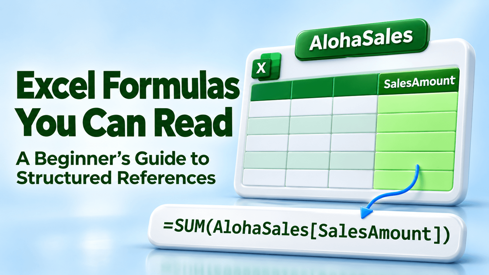


A formula like =SUM(D2:D4) tells Excel which cells to add. But when you return to that workbook next month, you may need to check the headings to remember what those cells contain.
Excel tables give you another way to write it:
=SUM(AlohaSales[SalesAmount])
That formula gives you a useful clue: add the SalesAmount column from the AlohaSales table.
The table and column names form a structured reference. Let’s build one with a small example you can try yourself.
Meet Aloha Print
Aloha Print is our fictional print shop. We’ll use three orders to practice calculating sales before any tax, shipping, or discounts.
On a blank worksheet, enter these headings in A1:D1 and the order details in rows 2–4. Leave the SalesAmount cells empty for now.
| Product | Quantity | UnitPrice | SalesAmount |
|---|---|---|---|
| T-shirts | 12 | 25 | |
| Mugs | 8 | 18 | |
| Tote bags | 5 | 40 |
Each row represents one order. Quantity is the number sold, and UnitPrice is the price of one item.
Start with an ordinary range
A range is a group of worksheet cells. Our example occupies A1:D4.
In D2, enter:
=B2*C2
The asterisk means multiply. Here, Excel multiplies 12 by 25 to give 300.
Copy that formula down to D3 and D4. The other sales amounts are 144 and 200.
In F1, type Total sales. In F2, enter:
=SUM(D2:D4)
The total is 644.

This is a valid way to calculate the orders. Now let’s build the same example using names that explain the calculation.
Turn the list into an Excel table
On a second worksheet, enter the same headings and order details in A1:D4. Leave D2:D4 empty again so we can create the table formula from scratch.
- Select A1:D4, then choose Insert → Table. In Windows, Ctrl+T is another way to create the table.
- In the Create Table dialog, check the selected range and select My table has headers.
- In What is the name of your table?, enter AlohaSales, then choose OK.

Use AlohaSales without a space. That name identifies this table within the workbook.
If your Create Table dialog does not show a name field, create the table first. Then click inside it and use Table Design → Table Name to name it AlohaSales. On Mac, look for the Table tab.
Calculate each order using column names
In D2, enter:
=[@Quantity]*[@UnitPrice]
Read it as: “Multiply this row’s Quantity by this row’s UnitPrice.”
- Quantity and UnitPrice are the column headings.
- The brackets identify the column references.
- The @ symbol means this row.
Press Enter. Excel normally fills the formula through the table’s SalesAmount column. This is called a calculated column: one calculation is applied to each row. Microsoft’s calculated-column guide explains the behavior in more detail.
You should see the same three results: 300, 144, and 200.

Add the whole column by name
On this second worksheet, type Total sales in F1. In F2, enter:
=SUM(AlohaSales[SalesAmount])
Here’s how to read it:
- SUM adds the numbers.
- AlohaSales identifies the table.
- [SalesAmount] identifies the data in that table column.
There’s no @ in this reference because we want the whole SalesAmount data column, rather than one row. The total is still 644.
These names can make formulas easier to follow when you review your work or hand the workbook to someone else. Microsoft’s structured-reference guide covers the syntax and additional options.
Add one more order
Now Aloha Print receives an order for six more T-shirts at 25 each. That order adds 150, so the new total should be 794.
On your ordinary-range worksheet, enter the order in A5:C5 and put =B5*C5 in D5. A formula that still reads =SUM(D2:D4) excludes D5. You would need to extend it to =SUM(D2:D5) to include that order.

On your table worksheet, type the same order directly below the last table row, starting in A5. With Excel’s normal table-expansion and formula-fill behavior, the table grows to include the order and fills in its SalesAmount.
The total formula stays:
=SUM(AlohaSales[SalesAmount])
Because the new row is now part of the table, that reference includes its 150. Your total becomes 794.

Check that the new row really joined the table. A blank row between the table and a new order can leave that order outside it. If the table hasn’t expanded, use Table Design → Resize Table to include the intended range. See Microsoft’s guide to adding table rows.
If the SalesAmount formula doesn’t fill, confirm that it is a consistent calculated column and that automatic formula filling hasn’t been turned off.
Try it in a copy of your workbook
Choose a small list you use at work. Make a copy, turn the list into a table, and give it a descriptive name. Then total one numeric column using its name.
Add a test record and check both the new row and the total. Clearer formulas are useful, and checking the result is still part of the job.
Keep building your Excel skills
Want more practice with tables and formulas you can follow? My LearnFormula course, Excel Tables: Manage and Analyze Data Like a Pro, combines guided lessons with practice workbooks and quizzes. The full course is listed for 1 PD hour.
In the Using Structured References section, start with “Structured References Demystified: A Beginner's Guide” to build on what you’ve practiced here.
Complete the course’s requirements for its certificate, and confirm that it meets your professional body’s PD requirements. The hour applies to the full course, not this article or one lesson.
Let’s keep on learning. 🤙